Triple-negative breast cancer (TNBC) is one of the most aggressive forms of breast cancer because of its high risk of recurrence and limited treatment options. Unlike other breast cancer types, TNBC lacks three key molecular markers—estrogen receptor (ER), progesterone receptor (PR), and HER2—which are commonly targeted in standard therapies. As a result, patients are largely limited to chemotherapy, the current standard of care. Even then, outcomes remain poor: only about 20% of patients achieve a complete response, and those who do not face a significantly higher risk of recurrence and mortality (Nedeljković & Damjanović, 2019).
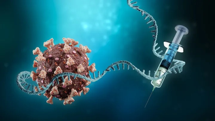
A promising new approach aims to overcome this limitation by turning the patient’s own tumor into a therapeutic target. While the concept of neoantigen mutation vaccines has existed for roughly 10-15 years and has been tested on cancers such as melanoma, vaccine efficacy against breast cancer is understudied. The paper “Individualized mRNA vaccines evoke durable T cell immunity in adjuvant TNBC” by Ugur Sahin et. al, aims to understand whether personalized neoantigen mRNA vaccines could generate strong and lasting immune responses specifically in patients with TNBC. These vaccines are designed using the unique genetic mutations found in an individual’s tumor, offering a highly tailored form of immunotherapy.
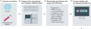
The concept hinges on neoantigens—mutated protein fragments that arise from cancer-specific DNA changes. Because these mutations are not found in normal cells, neoantigens are recognized as foreign by the immune system, making them ideal targets for immune attack. However, identifying which mutations will actually provoke a strong immune response is a major challenge, requiring sophisticated computational tools to predict which neoantigens are most likely to be effective.
In this study, 14 patients with TNBC who had already completed standard treatments—but remained at high risk of recurrence—were enrolled. For each patient, both tumor tissue and normal tissue were collected. Researchers then sequenced the tissue using Next Generation Sequencing (NGS). Next Generation Sequencing uses imaging to track fluorescently labeled nucleotides. The raw data is then processed by high powered computing software to align sequences to a reference genome. This process is much more cost and time efficient than alternative methods such as Sanger sequencing which can only handle smaller reading frames. The exact software was not specified by the study but some popular platforms are Integrative Genomics Viewer (IGV), used for the visualization and Illumina Connected Analytics, used to identify nucleotide discrepancies.
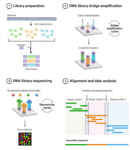
By highlighting genome misalignments, NGS aided researchers in identifying mutations unique to each patient’s tumor. From these mutations a select subset were chosen as vaccine targets based on their predicted ability to generate strong immune responses. Selected mutations were encoded into a personalized mRNA vaccine, with each vaccine containing instructions for up to 20 different neoantigens.
The mRNA design itself was carefully optimized. Structural features such as the 5′ cap, 3′ tail, and poly(A) sequence were modified to improve stability and enhance protein translation within immune cells. Once administered, the mRNA is taken up by dendritic cells, specialized immune cells that act as messengers. These cells translate the mRNA into protein fragments and present them to T cells, effectively “teaching” the immune system what to attack.
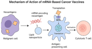
Importantly, the vaccine platform does more than simply deliver antigens, it also stimulates the immune system directly. The RNA–lipoplex (RNA–LPX) technology uses uridine-containing mRNA that activates Toll-like receptors (TLRs), proteins that normally detect viral infections. This triggers a type I interferon response, an early antiviral defense mechanism. By mimicking a viral infection, the vaccine creates a strong activation signal alongside antigen presentation, leading to a powerful expansion of antigen-specific T cells, particularly CD8⁺ T cells, which are responsible for killing cancer cells.
Patients received their personalized vaccines approximately one year after completing chemotherapy and the average time to develop a vaccine was sixty-nine days. The full treatment consisted of eight doses. Doses were given weekly for the first six weeks and the last two were administered biweekly. The entire treatment period lasted 64 days. Researchers monitored immune responses by measuring CD4⁺ and CD8⁺ T-cell activity before vaccination and starting 7-14 days after the final dose. Specifically, T-cell activation was measured using assays such as IFNγ ELISpot and flow cytometry, which together show whether immune cells respond to tumor neoantigens. The IFNγ ELISpot assay works by detecting individual T cells that release interferon gamma (IFNγ) when exposed to vaccine-matched peptides; each signal corresponds to a single activated T cell, so the number of “spots” reflects the strength of the immune response. Flow cytometry complements this by labeling cells with fluorescent markers and passing them through a laser-based detector, allowing researchers to identify which T-cell populations (such as CD4⁺ or CD8⁺ T cells) are activated and whether they are producing cytokines after stimulation. Patient immune system responses were tracked all the way until six years following their treatment.
The results were striking. All 14 patients developed immune responses against at least one of their tumor-specific neoantigens. More than half of these responses were de novo, meaning they were newly generated by the vaccine rather than expansions of pre-existing immune cells. This finding is especially important, as it demonstrates that the vaccine can actively overcome the immune system’s natural tolerance to cancer by eliminating cancer completely.
In addition to generating new responses, the vaccines produced broad and multi-targeted immunity. Because each vaccine encoded multiple neoantigens, the immune system was trained to recognize several tumor-specific targets simultaneously. This reduces the likelihood that cancer cells can evade detection by mutating a single antigen. Even more encouraging, these T-cell responses were shown to be durable, persisting for months to years after vaccination. Such long-term immune activity raises the possibility of sustained protection against cancer recurrence.
The treatment was also well tolerated. The most commonly reported side effects—headache, fatigue, nausea, and chills—occurred within one to three days after vaccination and were generally mild. No severe adverse effects were reported, suggesting that the therapy is not only effective at stimulating the immune system but also safe for patients.
Overall, these findings suggest that personalized neoantigen mRNA vaccines can transform tumors that are typically “invisible” to the immune system into clear targets for attack. By inducing strong, multi-target, and long-lasting T-cell responses, this approach addresses several key challenges in cancer immunotherapy. It also highlights the evolving role of computational biology in medicine, as predicting effective neoantigens is essential to the success of these vaccines.
While the results are promising, important limitations remain. The study involved a small cohort of just 14 patients and did not include a large randomized control group. Additionally, while immune responses were robust, longer-term clinical outcomes such as recurrence rates and overall survival require further investigation. The process of designing and manufacturing personalized vaccines is also time-intensive and costly, though advances in technology may help streamline these steps in the future.
Nevertheless, this study represents a significant step forward. It demonstrates that individualized mRNA vaccines are not only feasible but also capable of generating meaningful immune responses in patients with difficult-to-treat cancers like TNBC. As larger clinical trials are conducted and the technology continues to improve, personalized cancer vaccines may become a powerful new tool—one that turns each patient’s unique tumor biology into a blueprint for their own cure.
References:
Illumina. 2022. Sequencing Technology | Sequencing by synthesis. www.illuminacom. https://www.illumina.com/science/technology/next-generation-sequencing/sequencing-technology.html.
Malla R, Srilatha Mundla, Farran B, Ganji Purnachandra Nagaraju. 2024. mRNA vaccines and their delivery strategies: A journey from infectious diseases to cancer. Molecular therapy. 32(1):13–31. doi:https://doi.org/10.1016/j.ymthe.2023.10.024.
Nedeljković M, Damjanović A. 2019. Mechanisms of Chemotherapy Resistance in Triple-Negative Breast Cancer—How We Can Rise to the Challenge. Cells. 8(9):957. doi:https://doi.org/10.3390/cells8090957.
Sahin, U., Schmidt, M., Derhovanessian, E. et al. Individualized mRNA vaccines evoke durable T cell immunity in adjuvant TNBC. Nature 651, 1088–1096 (2026). https://doi.org/10.1038/s41586-025-10004-2